Cusp and Generalized Hopf bifurcations
Here the bifurcations concern singularities with co-dimension greater than 1.
These are only unfolded by local families that depend on more than 1
parameter.
Cusp bifurcation
Given
 a smooth vector field with a cusp singularity at the
origin. Then
a smooth vector field with a cusp singularity at the
origin. Then
 but
but
 =
= =
= and
and
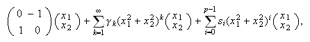
 has normal form (with
 and
and
 ).
). The
local
family
The
local
family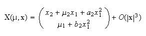 is
a versal unfolding of the cusp singularity above. (Note that the cusp
singularity requires at least two parameters to completely unfold it).
Considering this local family
is
a versal unfolding of the cusp singularity above. (Note that the cusp
singularity requires at least two parameters to completely unfold it).
Considering this local family
 ,
under some conditions (not shown here) in particular about parameters, it is
possible to generate three bifurcation types: (1) Saddle
node, (2) Hopf bifurcation, (3)
Saddle connection.
,
under some conditions (not shown here) in particular about parameters, it is
possible to generate three bifurcation types: (1) Saddle
node, (2) Hopf bifurcation, (3)
Saddle connection.
Generalized Hopf bifurcations
Generalized Hopf bifurcations. (Takens 1973b, Guckenheimer
& Holmes 1983, Arrowsmith & Place 1990). Here, we describe the
generalized Hopf singularity of type
 .
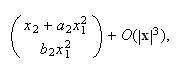
The vector field in the previous co-dimension 1 Hopf bifurcation was obtained
by posing
.
The vector field in the previous co-dimension 1 Hopf bifurcation was obtained
by posing
 in the normal
form
in the normal
form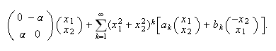 If
a degeneracy is introduced by posing
If
a degeneracy is introduced by posing
 =
= =
= =
= =
= with
with
 ,
then the system above is said to have a generalized Hopf
singularity of type
,
then the system above is said to have a generalized Hopf
singularity of type
 at
at
 =
= .
(Note that a co-dimension
.
(Note that a co-dimension
 Hopf singularity is said to be of type
 ).
The framework of the generalized Hopf singularity highlights
the relationship between the degeneracy of a singularity and the number of
parameters contained in its versal unfolding.
).
The framework of the generalized Hopf singularity highlights
the relationship between the degeneracy of a singularity and the number of
parameters contained in its versal unfolding.
If a Hopf singularity of type
 occurs, it is possible to reduce the system above to a simpler system.
Given
occurs, it is possible to reduce the system above to a simpler system.
Given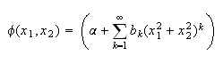 that
can also be
written:
that
can also be
written: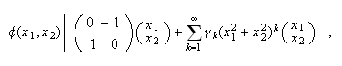 with
with
 =
= .
Because
.
Because
 >
> ,
we have
,
we have
 >
> for all
 enough close to the origin. Thus there exists a neighborhood of
 =
= on which the system is topologically equivalent to the (simpler)
vector
field:
on which the system is topologically equivalent to the (simpler)
vector
field: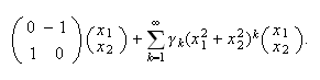 While
preserving the topological equivalence, we can replace
While
preserving the topological equivalence, we can replace
 by
by
 in the vector field above. Two cases are then possible according to a
singularity of the type:
in the vector field above. Two cases are then possible according to a
singularity of the type:
 or
or
 .
A versal unfolding for the vector field above can be obtained through the
following Takens theorem (1973b):
.
A versal unfolding for the vector field above can be obtained through the
following Takens theorem (1973b):
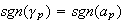
According to the sign of
 ,
the unfoldings of in this theorem gives two cases
,
the unfoldings of in this theorem gives two cases
 and
and
 .
Here, we only describe the first case
.
Here, we only describe the first case
 ,
and the latter case can be related to the other by a time reversal (so the
stabilities of fixed points and limit cycles are inverted). The formula in
this theorem, through the polar form
(
,
and the latter case can be related to the other by a time reversal (so the
stabilities of fixed points and limit cycles are inverted). The formula in
this theorem, through the polar form
( with here
 =
= ),
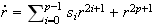
gives for
),
gives for
 the bifurcational behavior by using the equivalent equation:
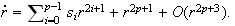 The behavior is independent of the terms of order
 (as described for the co-dimension 1 Hopf bifurcation), so it suffices to
consider
(as described for the co-dimension 1 Hopf bifurcation), so it suffices to
consider
 .
This equation in particular provides limit cycles. (1) For
.
This equation in particular provides limit cycles. (1) For
 =
= ,
by posing
,
by posing
 =
= ,
we obtain
,
we obtain
 ,
then a limit cycle occurs whose radius is
,
then a limit cycle occurs whose radius is
 only when
 <
< .
(2) For
.
(2) For
 =
= ,
by posing
,
by posing
 =
= ,
we obtain
,
we obtain
 and non-trivial zeros result from
 .
Then we obtain:
.
Then we obtain:
 If
If
 >
> and
and
 >
> (or
(or
 <
< ):
no limit cycle but a repelling spiral.
):
no limit cycle but a repelling spiral.
 If
If
 <
< and
and
 >
> :
two limit cycles.
:
two limit cycles.
 If
If
 <
< :
one limit cycle. (see
Fig.
:
one limit cycle. (see
Fig. below).
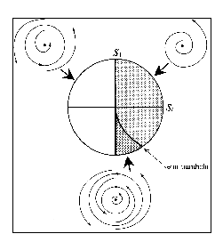 This
figure shows the bifurcation diagram for the type-(2,+) Hopf bifurcation. It
shows that a supercritical (subcritical) Hopf bifurcation occurs when
This
figure shows the bifurcation diagram for the type-(2,+) Hopf bifurcation. It
shows that a supercritical (subcritical) Hopf bifurcation occurs when
 increases through zero with
 <
< (subcritical with
 >
> ),
and a double limit cycle bifurcation occurs on the semi-parabola. If
),
and a double limit cycle bifurcation occurs on the semi-parabola. If
 decreases through the semi-parabola, a non-hyperbolic limit cycle occurs and
then divides into two hyperbolic cycles.
decreases through the semi-parabola, a non-hyperbolic limit cycle occurs and
then divides into two hyperbolic cycles.