
Some Examples of Pictures (Using MATLAB or c++):
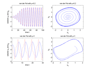
Fig.1 Van der Pol oscillator for μ=0.2 and μ=1.
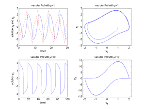
Fig.2 Van der Pol oscillator for μ=1 and μ=10.
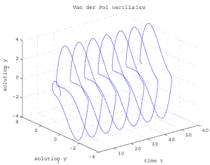
Fig.3 Van der Pol oscillator for μ=2.5, [t,y1,y2].
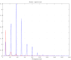
Fig.4 Power Spectrum of the variables y1 and y2 for the van der Pol oscillator for μ=2.5.
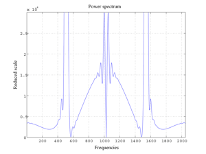
Fig.5 Power Spectrum (and lobes) of the logistic attractor for alpha=3.494.
Fig.6 Chua autonomous circuit (Chua attractor).
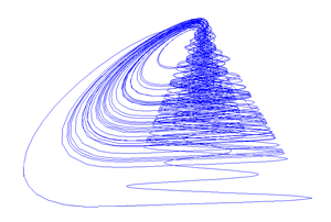
Fig.7 Colpitts oscillator (simple chaotic generator).
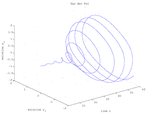
Fig.3b Van der Pol oscillator for μ=0.275, [t,y1,y2].
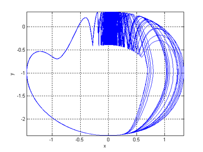
Fig.1.103. The first example of the specific equations undergoing the catastrophe was given by N. Gavrilov and A. Shilnikov:
(1). dx/dt = x (2+μ-β(x2+y2))+z2+y2+2y
(2). dy/dt = -z3-(1+y)(z2+y2+2y)-4x+μy
(3). dz/dt = (1+y)z2+x2+η
With β=10, μ=0.456, η=0.0357
A bleu sky orbit underlying catastrophe, i.e. blue sky bifurcation. For [x,y,z]. (Azimut=0°, Elevation=0°).
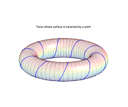
Fig.8 Torus (genus 1) whose surface is traversed by a point trajectory.
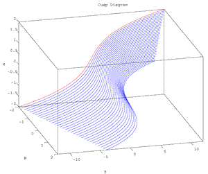
Fig. Cusp Diagram, which can be given by a system such as fγ,μ(x)=γ+μx-x3=0.
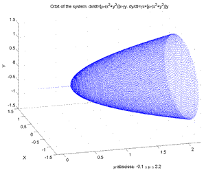
Fig. Orbit and Hopf Bifurcation of the Nonlinear Dynamical System: dz/dt= (μ+iγ)z-z|z|2 z=complex: (Hopf), γ=fixed.μ=-0.2,..,2.2 [μ-abscissa, x1, x2].
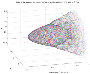
Fig.8bis Orbit and Bifurcations of a Nonlinear Dynamical System according to μ, γ. (γ=-1,...,1, μ=-0.5,..,3). [μ-abscissa, x1, x2]. ATTENTION: Consider as an exercise the question: Is this simulation valid or not? (see correspond. m-file, "Dynamic2.m").
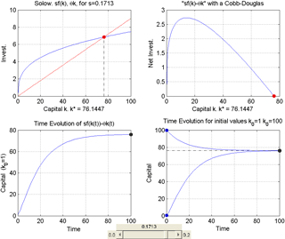
Fig.9 Steady State of the Reference Solow Model (1956) when the rate s varies. Investment: sf(k), µk; Net-Invest.: sf(k)-µk; Time Evolution of sf(k(t))-µk(t); Time Evolution of capital for two initial conditions.
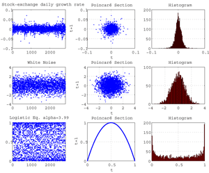
Fig.10 Poincaré sections and histograms of stock-index increments, a white noise, a chaotic dynamic (i.e. quadratic map).
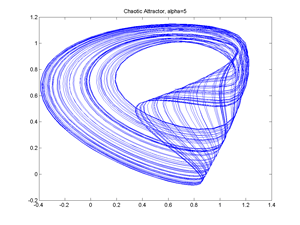
Fig.11 Delay Model and Logistic equation, Chaotic Attractor (ref. to Medio.1992).
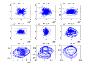
Fig.12 (Delay model with May eq.). Projections of reconstructed attractor by using Singular Spectrum Analysis. Fig. shows pairwise components of matrix XC. [X=Trajectory matrix,Transp(X); V=Transp(X)(X), c=Eigenvectors of V, b=Eigenvalues of V, Vc, b.c, V=Tranp(Xc)(Xc), Xc=reconstructed attractor projections]. (By other software)
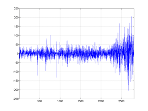
Fig.13 2806 First-differences of the cac40 stock-index (Jan 1988 - april 1998).
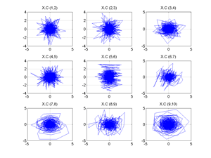
Fig.14 Projections of the reconstructed series by the SSA method. Pairwise components of the matrix XC (by disregarding time).
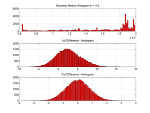
Fig.15 Distributions of a digital (pseudo) fractional Brownian Motion and its 1st and 2nd differences (Hurst exponent =0.8).
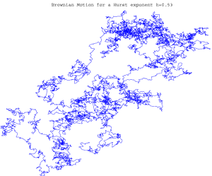
Fig.16 Walk of a digital (pseudo) fractional Brownian motion for H=0.53 in a plane with 10000 steps. Observe the loops and the way in which the plane is blackened by the walk of the fractional brownian motion.
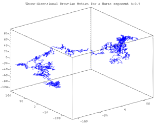
Fig. 16bis Walk of a digital (pseudo) Brownian motion for H=0.5 in a 3-dimensional Euclidean space with 10000 steps. Observe the loops and the way in which the volume is blackened by the fractional brownian motion walk..
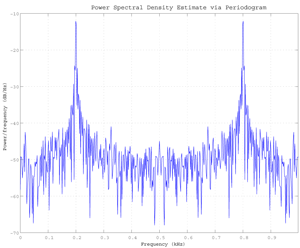
Fig. Power Spectrum Density via Periodogram of a 200 Hz signal embedded in additive noise using the default window.
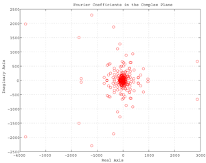
Fig. Fundamental tool of signal processing is FFT (or fast Finite Fourier Transform). Here is an example using FFT applied to sunspot periodicity that shows Fourier coefficients in the complex plane. (Sunspot activity over the last 300 years)
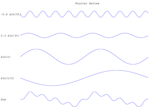
Fig. Wave functions whose sum is shown at bottom.
Reminder: An arbitrary periodic function (even discontinuous) can be represented by a sum of sinusoids of different frequencies, each one is endowed with a coefficient. The set of these coefficients allows to reconstitute the initial function or series. This is the Fourier series principle. It allows to transform a time series or function into a series of independent (differential) equations. Each one of these equations shows the chronological evolution of the coefficients of one of the sinusoids which will compose the initial series. Fourier series can be written for example without cosine: f(x)=c1.sinφ1(x)+c2.sinφ2(x)+c3.sinφ3(x)+... ; e.g. f(x)=sin(x)+(1/a)sin(a.x)+(1/b)sin(b.x)+... , the coefficients are here (1,1/a,1/b,...). Illustration is given in the above picture where f(x)=(-0.4sin(5x))+(0.3sin (3x))+(sin (x))+(sin(x/2)); this series is written as the sum of sinusoidal functions. At a given frequency, Fourier coefficient measure is done by computing the integral of function or series.
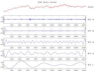
Fig. Five Morlet wavelet transforms of a stock-index.
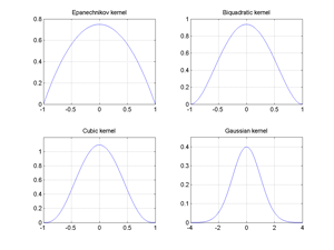
Fig.17 Epanechnikov, Biquadratic, Gaussian and Cubic kernels.
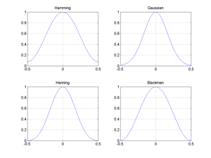
Fig.17bis Hamming, Gaussian, Blackman, Hanning windows.
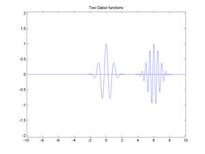
Fig.18 Two Gabor functions (also named Gabor atoms).
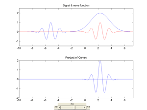
Fig.19 Convolution of an arbitrary signal with a wave function which moves along the signal. A convolution of two functions f and g can be written for instance as follows: f * g = Integral of [ g(s) . f(t-s) ] ds.
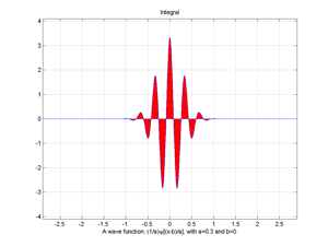
Fig.20 Area of a wave function.
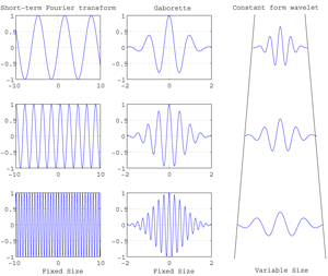
Fig.21 Distinction of the different window mechanisms by type of Transformation. Types of transformation: 1.Short-term Fourier: Fixed size, 2.Gabor function: Fixed size, 3.Constant form wavelet: Variable size.
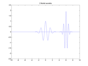
Fig.22 Two Morlet Wave functions.
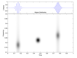
Fig.23 Wigner-Ville Time-Frequency Distribution of two Gabor atoms (colormap gray scale version). Note the interference component.
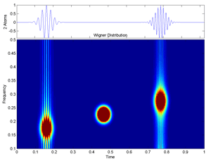
Fig.22 Wigner-Ville Time-Frequency Distribution of two Gabor atoms (colormap jet version).
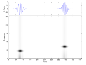
Fig.24 Cohen Time-Frequency Distribution of two Gabor atoms. The Alias-Free Generalized Time-Frequency Distribution provides analogous results.
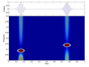
Fig.25 Alias-Free Generalized Time-Frequency Distribution of two Gabor atoms.
Fig.26 Time-Frequency Spectrogram of the signal "transients".
Fig.27 Wigner-Ville Time-Frequency Distribution of the signal "transients".
Fig.28 Cohen Time-Frequency Distribution of the signal "transients".
Fig.29 Cohen Time-Frequency Distribution of the signal "transients" (jet version).
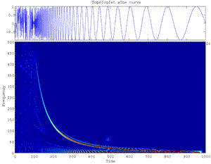
Fig.30 Cohen Time-Frequency Distribution of the Topologist's sine curve.
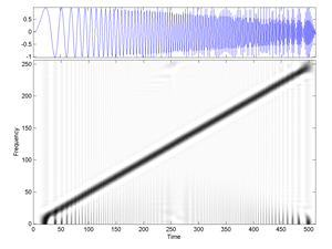
Fig.31 Cohen Time-Frequency Distribution of the signal "linchirp".
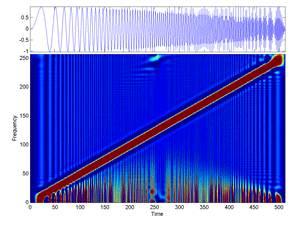
Fig.31b Cohen Time-Frequency Distribution of the signal "linchirp" (jet version).
Fig. Via Wavelab802, for the signal transients
, here are Compared Images of Continuous Wavelet Transforms by using: (a) Gauss, (b) DerGauss, (c) Sombrero, (d) Morlet. (The images are displayed in the Time-Frequency plane).
Fig. The lower-right image (d) of the previous Fig. is enlarged here; The wavelet used is that of Morlet via Wavelab802. One slightly perceives cross structures at high frequencies. (Continuous Wavelet Transform of the signal transients
). (Gray scale version).
Fig.32 Same as above but by using another m-file cwt.m
and displaying parametrization, which is not that of Wavelab802. The cross structures are easier to perceived here. (Image of a Continuous Wavelet Transform of the signal transients
). (Gray scale version).
Fig.33 Same as above but with Colormap Hot
.
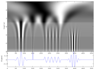
Fig. Image of a Continuous Wavelet Transform of an arbitrary signal that consists of. (1) two slighly different Gabor atoms whose internal frequencies progressively increase, (2) A dirac, (3) A sinusoid, (4) A noise that increases at each sequence repetition.The wavelet is a Sombrero. (See movie)
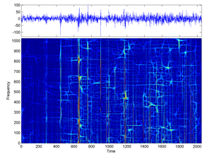
Fig.34 Cohen Time-Frequency Distribution of 2048 Cac40 first-difference daily values (for sigma large).
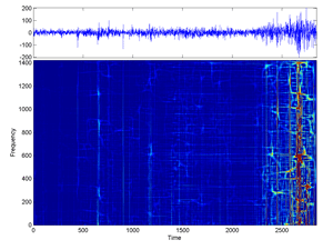
Fig.35 Cohen Time-Frequency Distribution of 2847 Cac40 first-differences (for sigma large).
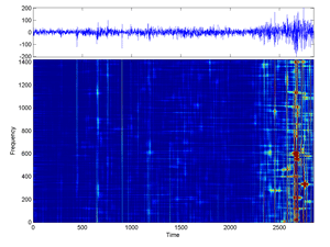
Fig.36 Cohen Time-Frequency Distribution of 2847 Cac40 first-differences daily values (for smaller sigma).
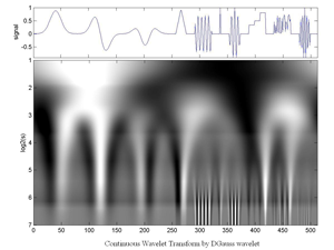
Fig.5.40 Continuous Wavelet Transform (by Gauss-Derivative Wavelet) of an artificial Signal that consists of:
(1) a Gauss window,
(2) its Derivative x104,
(3) its second derivative,
(4) a triangular fct.
(5) a short sinusoid,
(6) a Dirac,
(7) a Morlet wavelet,
(8) a short staircase,
(9) a short random series,
(10) an increasing then decreasing oscillating structure. Length=512.
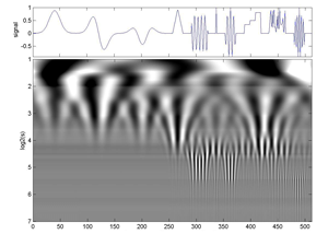
Fig.5.41 Same signal as before but the analysing wavelet is a morlet. It is a Continuous Morlet Wavelet Transform.
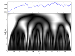
Fig.37 Image of a (Time-Frequency) Continuous Wavelet Transform of 2048 Cac40 daily values.
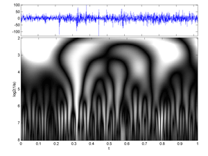
Fig.38 Image of a (Time-Frequency) Continuous Wavelet Transforms of 2048 Cac40 first-differences daily values.
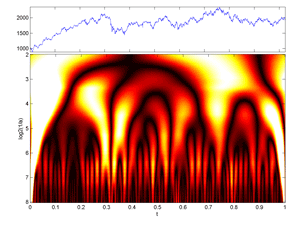
Fig.39 Image of a (Time-Frequency) Continuous Wavelet Transform of 2048 Cac40 daily values (colormap hot version).
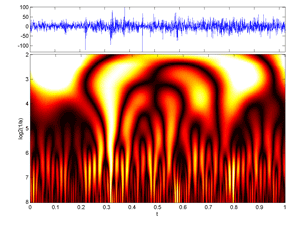
Fig.40 Image of a (Time-Frequency) Continuous Wavelet Transform of 2048 Cac40 first-differences daily values (colormap hot version).
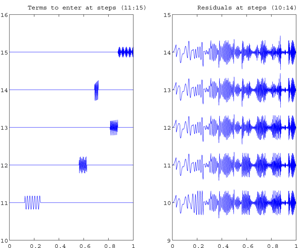
Fig. Example of animation of an Atomic Decomposition into Cosine Packets by Matching Pursuit of the signal Linchirp
, 512 data..
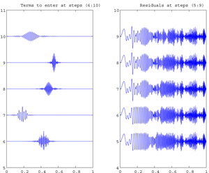
Fig. Example of animation of an Atomic Decomposition into Wavelet Packets by Matching Pursuit of the signal Linchirp
, 512 data..
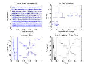
Fig.41 Best Basis for the signal "transients": 1.Cosine packet decomposition, 2.Cosine packet Best Basis Tree, 3.Plot of CP Heisenberg Boxes in the Phase plane, 4.Image of CP Heisenberg Boxes in the Time-Frequency plane.
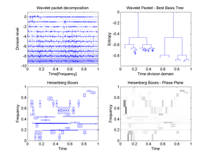
Fig.42 Best Basis for the signal "transients": 1.Wavelet packet decomposition, 2.Wavelet packet Best Basis Tree, 3.Plot of WP Heisenberg Boxes in the Phase plane, 4.Image of WP Heisenberg Boxes in the Time-Frequency plane.
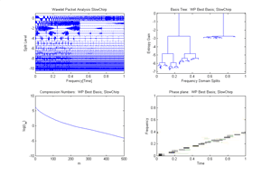
Fig.43 Example of Best basis and WP decomposition of the signal "slow shirp": 1.Wavelet packet decomposition, 2.Wavelet packet Best Basis Tree, 3.Compression Numbers, 4.Image of WP best basis Heisenberg Boxes in the Phase plane.
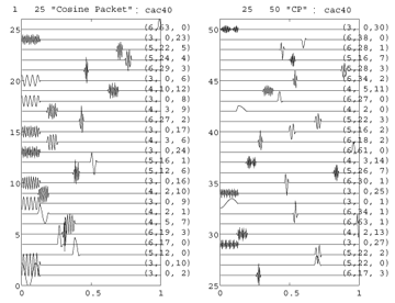
Fig.44 Example of 50 cosine packets repertories for a stock-index.
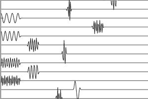
Fig.45 Detail of the cosine packet repertories above.
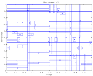
Fig.46 Heisenberg Boxes of Matching Pursuit Fourier Atoms in the Time-Frequency plane for a stock-index sample (512 data).
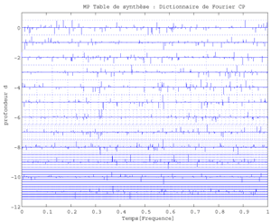
Fig.47 Fourier Dictionary for a longer stock-index sample (x-axis:Time-Frequency; y-axis: Depth of the dictionary).
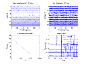
Fig.48 1.Matching Pursuit Synthesis Table (Cosine Packet Dictionary), 2.MP Residuals, 3.Compression Numbers, 4.Heisenberg Boxes in the Phase phane (Signal: a short stock-index sample).
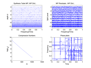
Fig.49 1.Matching Pursuit Synthesis Table (Wavelet Packet Dictionary), 2.MP Residuals, 3.Compression Numbers, 4.Heisenberg Boxes in the Phase phane (Signal: a short stock-index sample).
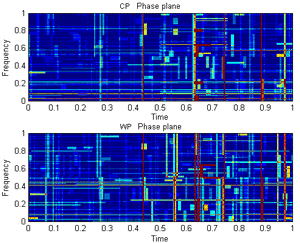
Fig.50 Images of matching Pursuit CP and WP Heisenberg boxes for a same signal (a stock index, 2048 Data).
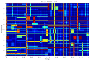
Fig.51 Image of Heisenberg Boxes of Matching Pursuit Fourier Atoms in the Time-Frequency plane for a stock-index sample (512 data).
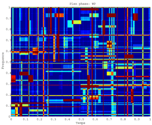
Fig.52 Image of Heisenberg Boxes of Matching Pursuit wavelet atoms in the Time-Frequency plane for a stock-index sample (512 data).
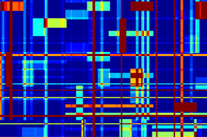
Fig.53 Detail of the previous picture.
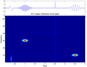
Fig.54 Wigner Distribution of Matching Pursuit Time-frequency atoms in the Phase plane of an arbitrary signal (according to Mallat-Zhang developments,98).
The signal is composed of: 1.One short sine (at the beginning), 2.Two Gabor functions, 3.One dirac function, 4.A noise along the signal.
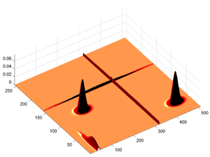
Fig.55 Same Data as before but shown in three dimension. Note the transverse line corresponding to the noise that has been added to the signal.
Fig.56 Wigner Distribution of Matching Pursuit waveform atoms in the Time-Frequency plane for the signal "transients" (512 data).
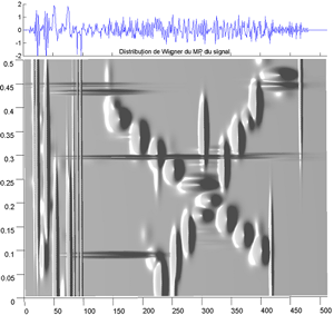
Fig.56 Same as before but with the relief expressing the amplitude.
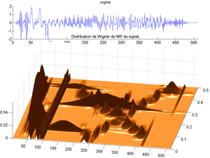
Fig.58 Same as before but with relief, elevation and azimut.
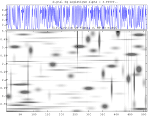
Fig.59 Wigner Distribution of Matching Pursuit waveform atoms in the Time-Frequency plane for the logistic map in the chaotic domain (512 data).
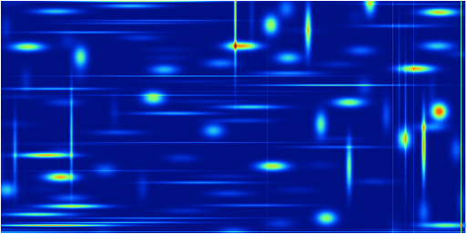
Fig.60 Same as before (colormap jet version).
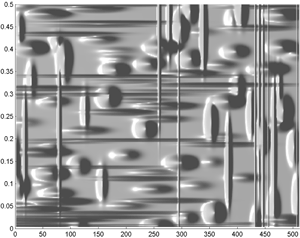
Fig.61 Same as before with relief.
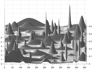
Fig.62 Same as before with relief and elevation (and azimut 0°).
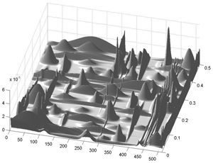
Fig.63 Same as before with relief, elevation and azimut.
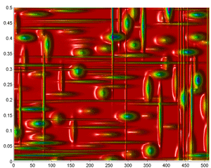
Fig.64 Wigner Distribution of Matching Pursuit waveform atoms in the Time-Frequency plane for the logistic map in the chaotic domain (512 data).
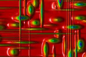
Fig.65 Detail of the previous picture (colormap HSV).
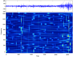
Fig.66 Wigner Distribution of Matching Pursuit Time-Frequency atoms in the phase plane for eleven years of a stock-index.
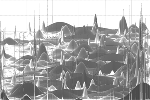
Fig.67 Energy Distribution of Matching Pursuit Time-Frequency atoms in the Phase Space for eleven years of a stock-index (elevation 35°, azimut 0°).
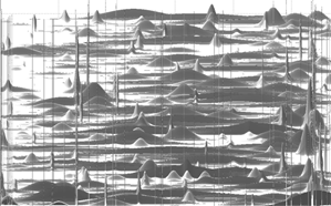
Fig.68 Wigner Distribution of Matching Pursuit Time-Frequency atoms in the Phase Space for eleven years of a stock-index (elevation 75°, azimut 0°).
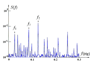
Fig.69 Spectrum of a quasiperiodic signal for three immeasurable frequencies observed in the R-B instability, Ra/Rac=42,3 (the spectral scale is logarithmic). Before this value, several (Hopf) bifurcations occurred for lower values of Ra/Rac. (ref. to J.Gollub & S.Benson).
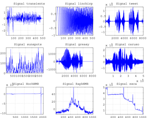
Fig. Some well-known Signals: (1) transients.asc; (2) linchirp.asc;(2) tweet.asc; (2) sunspots.asc; (2) greasy.asc; (2) caruso.asc; (2) HochNMR.asc; (2) RaphNMR.asc; (2) esca.asc.
Fig.a Transient Signal (512 data).
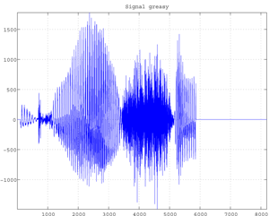
Fig.b Greasy signal (8192 data).
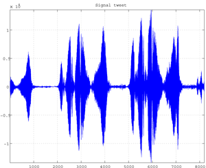
Fig.c Tweet Signal (8192 data).
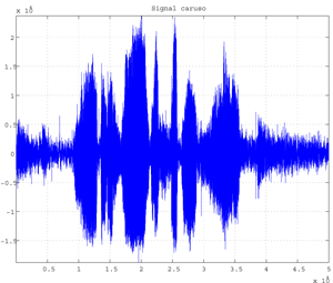
Fig.d Caruso sSgnal (50.000 data).
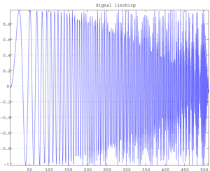
Fig.d Linchirp Signal (512 data).
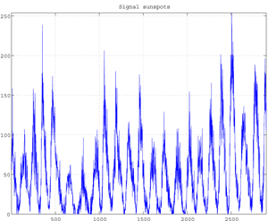
Fig.e Sunspots Signal (2899 data).
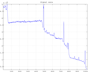
Fig.f Esca Signal (elevation 35°, azimut 0°).
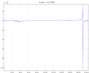
Fig.g HochNMR Signal (2048 data).
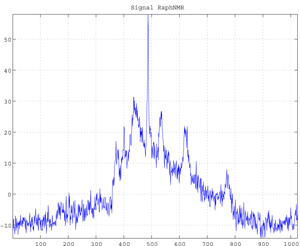
Fig.g RaphNMR Signal (1024 data).
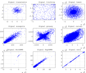
Fig. First returm maps for well-known Signals: (1) transients.asc;(2) linchirp.asc; (3) tweet.asc; (4) sunspots.asc; (5) greasy.asc; (6) caruso.asc; (7) HochNMR.asc; (8) RaphNMR.asc; (9) esca.asc.
Note that here the use of first return map does not presage of its utility but has a rather didactic sense.