
A Few Examples of Pictures (Using MATLAB or c++):
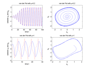
Fig.1.116 Van der Pol oscillator for μ=0.2 and μ=1.
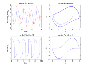
Fig.1.117 Van der Pol oscillator for μ=1 and μ=10.
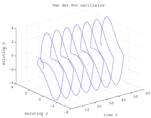
Fig.1.118 Van der Pol oscillator for μ=2.5, [t,y1,y2].
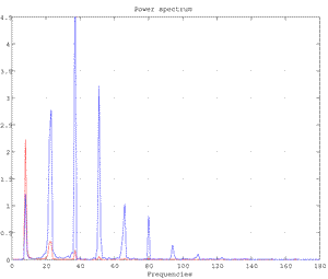
Fig.4 Power Spectrum of the variables y1 and y2 for the van der Pol oscillator for μ=2.5.
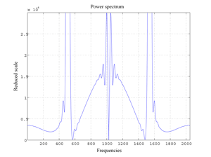
Fig.209 Power Spectrum (and lobes) of the logistic attractor for alpha=3.494.
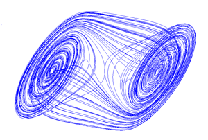
Fig.1.33 Chua autonomous circuit (Chua attractor).
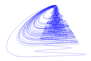
Fig.1.35 Colpitts oscillator (simple chaotic generator).
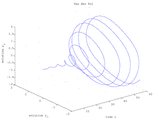
Fig.1.117d Van der Pol oscillator for μ=0.275, [t,y1,y2].
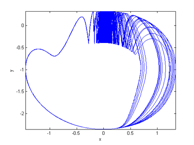
Fig.1.103. The first example of the specific equations undergoing the catastrophe was given by N. Gavrilov and A. Shilnikov:
(1). dx/dt = x (2+μ-β(x2+y2))+z2+y2+2y
(2). dy/dt = -z3-(1+y)(z2+y2+2y)-4x+μy
(3). dz/dt = (1+y)z2+x2+η
With β=10, μ=0.456, η=0.0357
A bleu sky orbit underlying catastrophe, i.e. blue sky bifurcation. For [x,y,z]. (Azimut=0°, Elevation=0°).
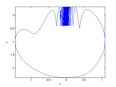
Fig.1.103. Blue sky orbit (N. Gavrilov and A. Shilnikov).