A Few Examples of Pictures (Using MATLAB or c++):
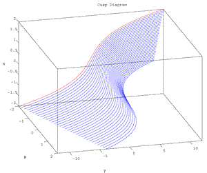
Fig. Cusp Diagram, which can be given by a system such as fγ,μ(x)=γ+μx-x3=0.
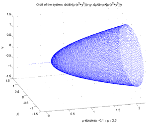
Fig.1.4d Orbit and Hopf Bifurcation of the Nonlinear Dynamical System: dz/dt= (μ+iγ)z-z|z|2 z=complex: (Hopf), γ=fixed.μ=-0.2,..,2.2 [μ-abscissa, x1, x2].
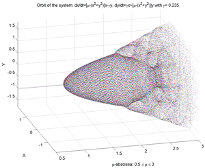
Fig.8bis Orbit and Bifurcations of a Nonlinear Dynamical System according to μ, γ. (γ=-1,...,1, μ=-0.5,..,3). [μ-abscissa, x1, x2]. ATTENTION: Consider as an exercise the question: Is this simulation valid or not? (see correspond. m-file, "Dynamic2.m").
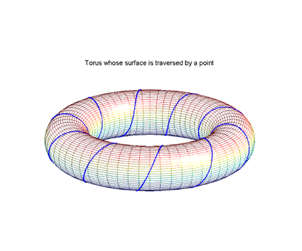
Fig.1.49 Torus (genus 1) whose surface is traversed by a point trajectory.
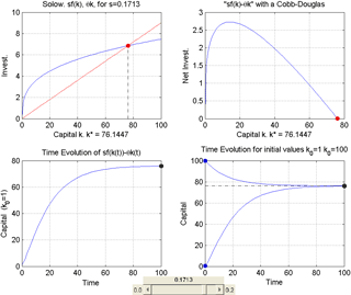
Fig.9 Steady State of the Reference Solow Model (1956) when the rate s varies. Investment: sf(k), µk; Net-Invest.: sf(k)-µk; Time Evolution of sf(k(t))-µk(t); Time Evolution of capital for two initial conditions.
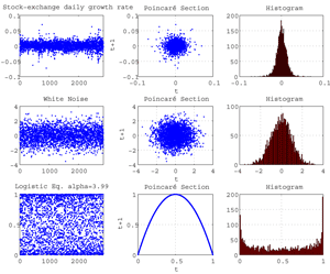
Fig.10 Poincaré sections and histograms of stock-index increments, a white noise, a chaotic dynamic (i.e. quadratic map).
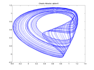
Fig.2.8 Delay Model and Logistic equation, Chaotic Attractor (ref. to Medio.1992).
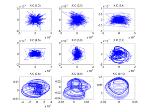
Fig.2.12 (Delay model with May eq.). Projections of reconstructed attractor by using Singular Spectrum Analysis. Fig. shows pairwise components of matrix XC. [X=Trajectory matrix,Transp(X); V=Transp(X)(X), c=Eigenvectors of V, b=Eigenvalues of V, Vc, b.c, V=Tranp(Xc)(Xc), Xc=reconstructed attractor projections]. (By other software)
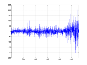
Fig.14 2806 First-differences of the cac40 stock-index (Jan 1988 - april 1998).
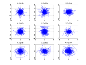
Fig.2.15 Projections of the reconstructed series by the SSA method. Pairwise components of the matrix XC (by disregarding time).
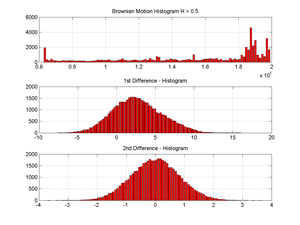
Fig.11 Distributions of a (pseudo) fractional Brownian Motion and its 1st and 2nd differences (Hurst exponent =0.8).
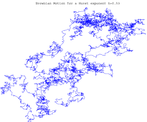
Fig.2.21 Walk of a digital (pseudo) fractional Brownian motion for H=0.53 in a plane with 10000 steps. Observe the loops and the way in which the plane is blackened by the walk of the fractional brownian motion.
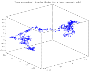
Fig.2.22 Walk of a digital (pseudo) fract.Brownian motion for H=0.5 in a 3-dimensional Euclidean space with 10000 steps. Observe the loops and the way in which the volume is blackened by the fractional brownian motion walk..
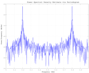
Fig. Power Spectrum Density via Periodogram of a 200 Hz signal embedded in additive noise using the default window.
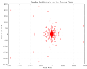
Fig. Fundamental tool of signal processing is FFT (or fast Finite Fourier Transform). Here is an example using FFT applied to sunspot periodicity showing the Fourier coefficients in the complex plane for the sunspot activity over the last 300 years.
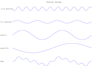
Fig. Wave functions whose sum is shown at bottom.
Reminder: An arbitrary periodic function (even discontinuous) can be represented by a sum of sinusoids of different frequencies, each one is endowed with a coefficient. The set of these coefficients allows to reconstitute the initial function or series. This is the Fourier series principle. It allows to transform a time series or function into a series of independent (differential) equations. Each one of these equations shows the chronological evolution of the coefficients of one of the sinusoids which will compose the initial series. Fourier series can be written for example without cosine: f(x)=c1.sinφ1(x)+c2.sinφ2(x)+c3.sinφ3(x)+... ; e.g. f(x)=sin(x)+(1/a)sin(a.x)+(1/b)sin(b.x)+... , the coefficients are here (1,1/a,1/b,...). Illustration is given in the above picture where f(x)=(-0.4sin(5x))+(0.3sin (3x))+(sin (x))+(sin(x/2)); this series is written as the sum of sinusoidal functions. At a given frequency, Fourier coefficient measure is done by computing the integral of function or series.
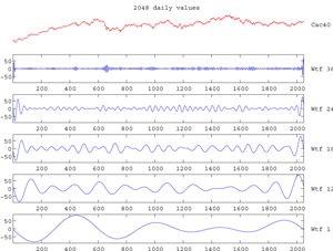
Fig. Five Morlet wavelet transforms of a stock-index.