
A Few Examples of Pictures (Using MATLAB or c++):
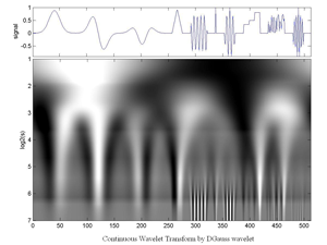
Fig.5.40 Continuous Wavelet Transform (by Gauss-Derivative Wavelet) of an artificial Signal that consists of:
(1) a Gauss window,
(2) its Derivative x104,
(3) its 2nd derivative,
(4) a triangular fct.
(5) a short sinusoid,
(6) a Dirac,
(7) a Morlet wavelet,
(8) a short staircase,
(9) a short random series,
(10) an increasing then decreasing oscillating structure.
Total length=512.
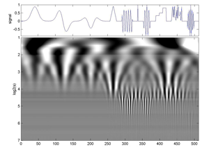
Fig.5.41 Same signal as before but the analysing wavelet is a morlet. It is a Continuous Morlet Wavelet Transform.
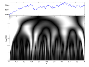
Fig.37 Image of a (Time-Frequency) Continuous Wavelet Transform of 2048 Cac40 daily values.
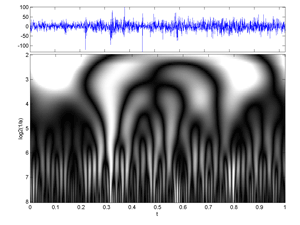
Fig.38 Image of a (Time-Frequency) Continuous Wavelet Transforms of 2048 Cac40 first-differences daily values.
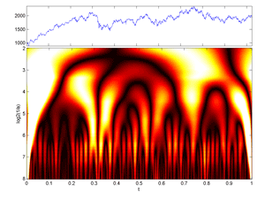
Fig.39 Image of a (Time-Frequency) Continuous Wavelet Transform of 2048 Cac40 daily values (colormap hot version).
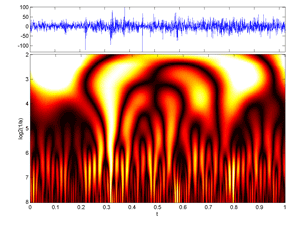
Fig.40 Image of a (Time-Frequency) Continuous Wavelet Transform of 2048 Cac40 first-differences daily values (colormap hot version).
Hereafter some Best Basis Cases for TRANSIENTS and SLOWSHIP Signals with:
1. Cosine packet decomposition, 2.Cosine packet Best Basis Tree, 3.Plot of CP Heisenberg Boxes in the Phase plane, 4.Image of CP Heisenberg Boxes in the Time-Frequency plane; then,
1.Wavelet packet decomposition, 2.Wavelet packet Best Basis Tree, 3.Plot of WP Heisenberg Boxes in the Phase plane, 4.Image of WP Heisenberg Boxes in the Time-Frequency plane.
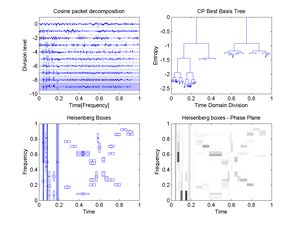
Fig.41 Best Basis for the signal "transients": 1.Cosine packet decomposition, 2.Cosine packet Best Basis Tree, 3.Plot of CP Heisenberg Boxes in the Phase plane, 4.Image of CP Heisenberg Boxes in the Time-Frequency plane.
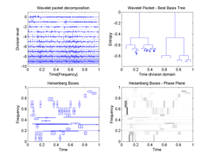
Fig.42 Best Basis for the signal "transients": 1.Wavelet packet decomposition, 2.Wavelet packet Best Basis Tree, 3.Plot of WP Heisenberg Boxes in the Phase plane, 4.Image of WP Heisenberg Boxes in the Time-Frequency plane.
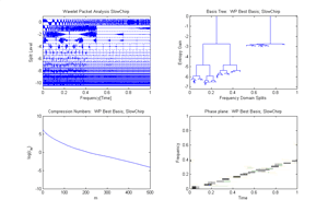
Fig.43 Example of Best basis and WP decomposition of the signal "slow shirp": 1.Wavelet packet decomposition, 2.Wavelet packet Best Basis Tree, 3.Compression Numbers, 4.Image of WP best basis Heisenberg Boxes in the Phase plane.